In this first blog post, I conduct some initial analyses of historical American presidential elections. Using popular vote data from 1948-2020 (provided by the course), I analyze how competitive elections are and the proportion of states that vote blue/red. My thanks to Matt Dardet for writing much of this code during and before our weekly section, as well as ShuXin Ho for helping me identify latitude/longitude loading bugs in my maps when we were initially building them in section.
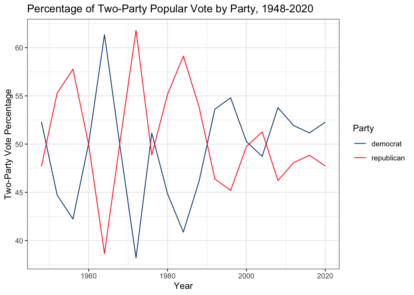
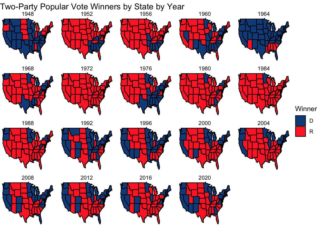
To answer this week’s questions, which focus on electoral competitiveness and historical voting patterns, we began by observing general trends in preference for either of the two major parties’ candidates between 1948 and 2020 at both the national and state level. For the former, we produced a line plot of the two-party vote share per party in each election. For the latter, we showed which candidate won each state in each election.
library(ggplot2)
library(maps)
library(tidyverse)
## ── Attaching core tidyverse packages ──────────────────────── tidyverse 2.0.0 ──
## ✔ dplyr     1.1.4     ✔ readr     2.1.5
## ✔ forcats   1.0.0     ✔ stringr   1.5.1
## ✔ lubridate 1.9.3     ✔ tibble    3.2.1
## ✔ purrr     1.0.2     ✔ tidyr     1.3.1
## ── Conflicts ────────────────────────────────────────── tidyverse_conflicts() ──
## ✖ dplyr::filter() masks stats::filter()
## ✖ dplyr::lag()    masks stats::lag()
## ✖ purrr::map()    masks maps::map()
## ℹ Use the conflicted package (<http://conflicted.r-lib.org/>) to force all conflicts to become errors
# Load in data
d_popvote <- read_csv('popvote_1948-2020.csv')
## Rows: 38 Columns: 9
## ── Column specification ────────────────────────────────────────────────────────
## Delimiter: ","
## chr (2): party, candidate
## dbl (3): year, pv, pv2p
## lgl (4): winner, incumbent, incumbent_party, prev_admin
##
## ℹ Use `spec()` to retrieve the full column specification for this data.
## ℹ Specify the column types or set `show_col_types = FALSE` to quiet this message.
# Create pivoted dataset and add winner column
d_popvote_wide <- d_popvote |>
  select(year, party, pv2p) |>
  pivot_wider(names_from = party, values_from = pv2p) |>
  mutate(winner = ifelse(democrat > republican, "D", "R"))
# Line plot demonstrating percentage of two-party popular vote per party
line_plot_win_trend <- d_popvote |>
  ggplot(mapping = aes(x = year, y = pv2p, color = party)) +
  geom_line() +
  scale_color_manual(values = c("dodgerblue4", "firebrick1")) +
  theme_bw() +
  labs(title = "Percentage of Two-Party Popular Vote by Party, 1948-2020",
       x = "Year",
       y = "Two-Party Vote Percentage",
       color = "Party")

# Loading state data for map and formatting for compatibility
states_map <- map_data("state")
d_pvstate_wide <- read_csv("clean_wide_state_2pv_1948_2020.csv")
## Rows: 959 Columns: 14
## ── Column specification ────────────────────────────────────────────────────────
## Delimiter: ","
## chr  (1): state
## dbl (13): year, D_pv, R_pv, D_pv2p, R_pv2p, D_pv_lag1, R_pv_lag1, D_pv2p_lag...
##
## ℹ Use `spec()` to retrieve the full column specification for this data.
## ℹ Specify the column types or set `show_col_types = FALSE` to quiet this message.
d_pvstate_wide$region = tolower(d_pvstate_wide$state)

# Creating new dataframe with winners highlighted
pop_2p_vote_w_state <- d_pvstate_wide |>
  left_join(states_map, by = "region") |>
  mutate(Winner = ifelse(D_pv2p > R_pv2p, "D", "R"))
## Warning in left_join(d_pvstate_wide, states_map, by = "region"): Detected an unexpected many-to-many relationship between `x` and `y`.
## ℹ Row 1 of `x` matches multiple rows in `y`.
## ℹ Row 1 of `y` matches multiple rows in `x`.
## ℹ If a many-to-many relationship is expected, set `relationship =
##   "many-to-many"` to silence this warning.
# Map of Two Party Popular Vote Winners by State
pop_2p_vote_winner_by_year_map <- pop_2p_vote_w_state |>
  ggplot(mapping = aes(x = long, y = lat, group = group)) + geom_polygon(aes(fill = Winner), color = "black") +
  scale_fill_manual(values = c("dodgerblue4", "firebrick1")) +
  facet_wrap(~year)+
  theme_void() +
  labs(title = "Two-Party Popular Vote Winners by State by Year",
       label = "Winner of State")

line_plot_win_trend
pop_2p_vote_winner_by_year_map
To further explore state competitiveness, especially in recent years, I also produced the following map demonstrating the average two-party popular vote margin in each state in each election following 2008. I define margin in this case as the difference between the percentage of a state’s voters who voted for the Democratic candidate and the percentage who voted for the Republican candidate. The result below averages this statistic across the 2012, 2016, and 2020 elections for each state. I chose this cutoff to reflect modern trends in state-party alignment, without bias from historical elections.
# Dataframe averaging the margin between Democratic and Republican vote share for 2012, 2016, and 2020 elections (by state)
pop_2p_vote_by_state_post2008 <- pop_2p_vote_w_state |>
  filter(year > 2008) |>
  mutate(margin = D_pv2p - R_pv2p) |>
  group_by(state, group, order, lat, long) |> # This particular order was necessary to avoid code bugs
  summarize(Average_Margin = mean(margin))
## `summarise()` has grouped output by 'state', 'group', 'order', 'lat'. You can
## override using the `.groups` argument.
# Mapping margin
map_pop_2p_vote_by_state_post2008 <- pop_2p_vote_by_state_post2008 |>
  ggplot(mapping = aes(x=long, y = lat, group = group)) +
  geom_polygon(aes(fill = Average_Margin), color = "black") +
  scale_fill_gradient2(high= "dodgerblue4",
                       mid = "white",
                       low = "firebrick1",
                       breaks = c(-50, -25, 0, 25, 50),
                       limits = c(-50,50)) +
  theme_void() +
  labs(title = "States by Average Two-Party Vote Share Margin post 2008 (in Percentage Points)",
       gradient = "Average Margin")


map_pop_2p_vote_by_state_post2008
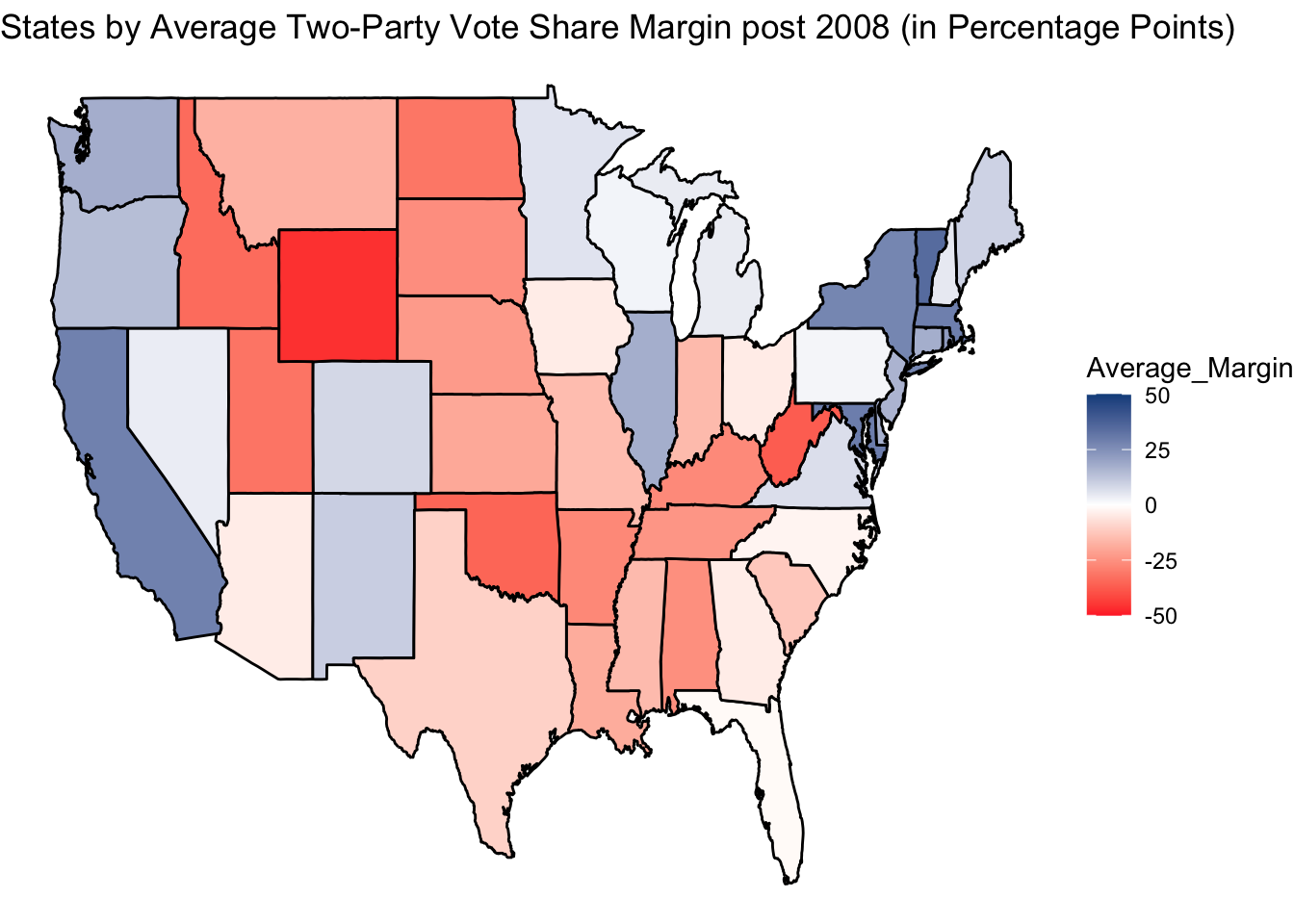
States that are more red on this map have consistently tended to overwhelmingly vote Republican, while those that are more blue have consistently voted overwhelmingly Democrat in recent years. While states like California and Wyoming appear to often regularly vote Democrat and Republican respectively, it is interesting to observe cases like Ohio or Michigan, which may tend to lean Republican or Democrat, but have a much smaller margin, indicating greater competitiveness.
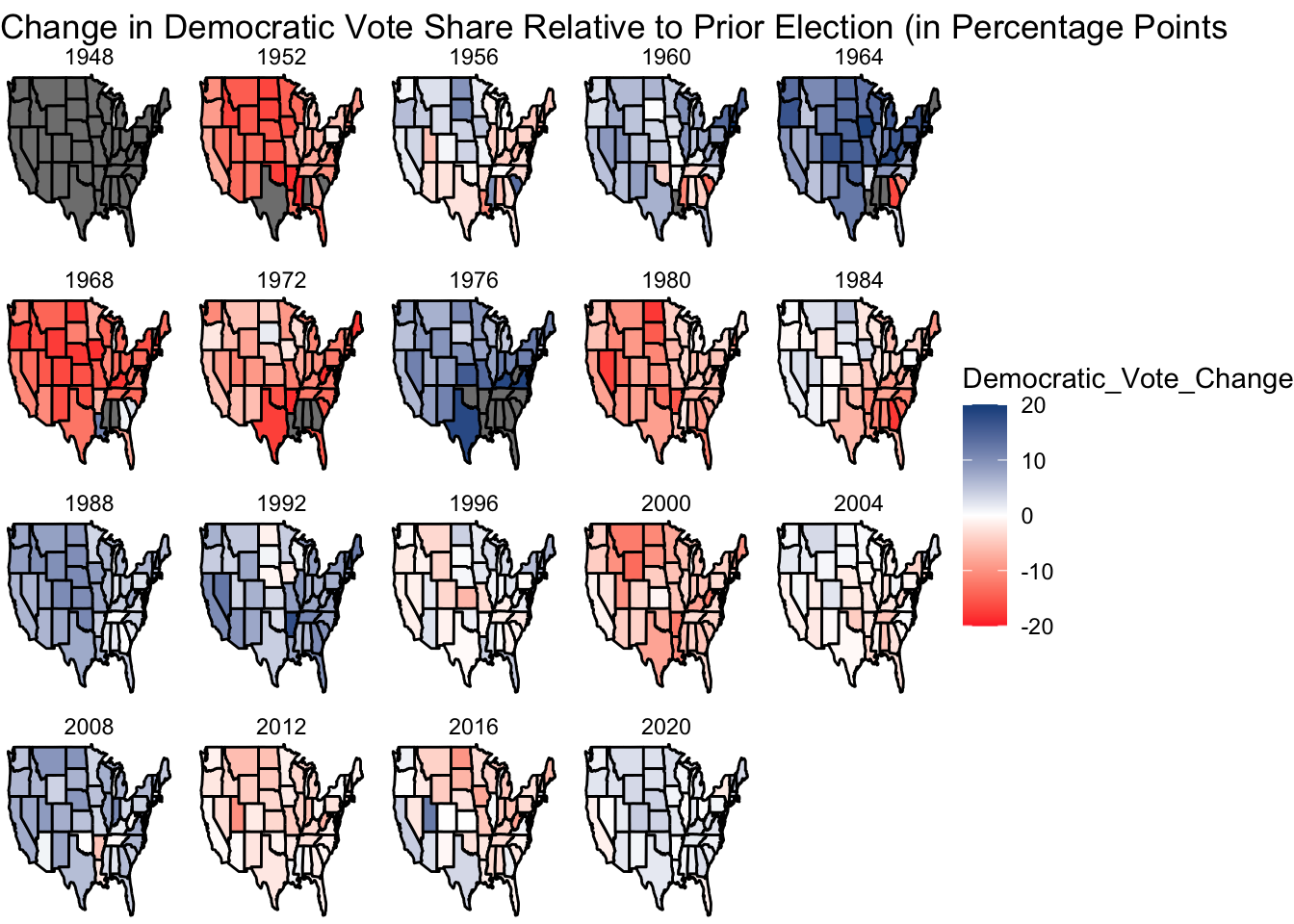
Then, to further understand what states have been battlegrounds, I created an additional map, which plots the degree to which a state’s Democratic vote share has changed compared to the prior election (Extension Option 3). Assuming that any declines correspond to an equal increase in Republican vote share and increases correspond to an equal decline in Republican vote share (ie: we ignore third party candidates for now), this map shows if a state has become “redder” or “bluer” since the previous election.
# New map measuring variation in Democratic vote share from previous election
swing_maps_data <- pop_2p_vote_w_state |>
  mutate(Democratic_Vote_Change = (D_pv2p) - (D_pv2p_lag1)) |>
  ggplot(aes(x = long, y = lat, group = group)) +
  geom_polygon(aes(fill = Democratic_Vote_Change), color = "black") +
  scale_fill_gradient2(low = "firebrick1",
                      mid = "white",
                      high = "dodgerblue4",
                      breaks = c(-20, -10, 0, 10, 20),
                      limits = c(-20,20)) +
  facet_wrap(~year) +
  theme_void() +
  labs(title = "Change in Democratic Vote Share Relative to Prior Election (in Percentage Points")

swing_maps_data
Questions:
1: How competitive are presidential elections in the United States?
Presidential elections in the United States are generally quite competitive. As seen in the line graph above, both primary parties appear to earn a significant share of votes in each election and the winning party changes quite frequently.
However, this competition appears to be driven by certain states that appear to be especially competitive. When focusing on recent elections, several states appear to consistently vote for one party, but others, especially as seen in the first map, may switch from selecting one party to the other
2: Which states vote blue/red and how consistently?
First, it is important to note that several states that consistently voted for one party in the earlier elections in this dataset tend to consistently vote for the opposite party in later years. This may be associated with the shifts in political preferences of each party during the latter half of the 20th century (1). Thus, when making predictions about consistency for upcoming elections, it is better to consider voting patterns in more recent years, to reflect more recent trends in voting.
Given this caveat, we can see that states in the south and middle of the United States have tended to consistently vote for Republicans, while those on the coasts and parts of the Midwest were more likely to vote for Democrats, when referencing the first map. However, certain states, often at the fringes of these geographic regions, were less consistent, such as Michigan, Pennsylvania, and Ohio. This is more clearly seen in the second and third maps, which do not show a clear pattern/preference in each of these states.
3: Extension: Plot a swing map for each year. Which states are/have been battleground states? Which states are no longer battlegrounds?
States on my swing map that appear to regularly alternate between increases (shown by a state being blue) and decreases (shown by a state being red) can be considered battleground states. These states have a lower chance of firmly voting for one party than states that are regularly only one color or appear to have little to no change relative to prior years (are white).
Based on this criteria, states like Michigan, Pennsylvania, Nevada, and Ohio appear to be swing states, including in recent years. This prediction also seems to align with the states that the US News has identified as swing states (2). However, Florida, on the other hand, appears to be an example of a state that is no longer a battleground, given that it has not changed much since the 2012 election.
Cited Sources
(1) Students of History. “The Great Switch: How Republicans and Democrats Flipped Ideologies.” Accessed September 7, 2024. https://www.studentsofhistory.com/ideologies-flip-Democratic-Republican-parties.; U.S. Embassy & Consulate in the Kingdom of Denmark. “Presidential Elections and the American Political System.” Accessed September 7, 2024. https://dk.usembassy.gov/usa-i-skolen/presidential-elections-and-the-american-political-system/.
(2) Davis Jr., Elliott. “7 States That Could Sway the 2024 Presidential Election.” US News & World Report, August 27, 2024. //www.usnews.com/news/elections/articles/7-swing-states-that-could-decide-the-2024-presidential-election.
Data Source
US Presidential Election Popular Vote Data from 1948-2020 (provided by the course)